Using the Automation1 Transformation Function for Five Axis Systems

The transformation functions in Automation1 implement rotation, mirror, and translation matrix operations. The functions can be used to transform coordinates on mechanical actuators that include rotary motion. Multiple rotation matrices can be configured using the TransformationConfigure() function for systems that have more than one rotary axis. A five‐axis system consisting of two rotary axes and three linear axes is an example of such a system (Figure 1). This application note will discuss the process of setting‐up the Transformation function for this type of application.

Theory of Operation

Five‐axis systems are capable of accessing any point on a hemisphere with a tool normal to the surface at the given point. Most 3D CAD tools can output tool paths that include the location on the surface in x/y/z coordinates along with the normal to the surface expressed as two angles (B and C in Figure 2).

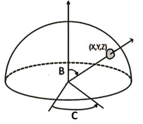
Aerotech’s transformation functions can take the part x/y/z positions and rotation angles and transform this information in real-time into position commands for the servo axes. Since the part positions are different from the servo system positions, two sets of axes must be used – one to define the part positions and the other to define the servo axes’ positions. The part‐axis system consists of three virtual axes and for this example we have named these axes x/y/z. The physical axes will be mapped to linear servo axes X/Y/Z and rotary axes B/C.

Right‐Hand Rule

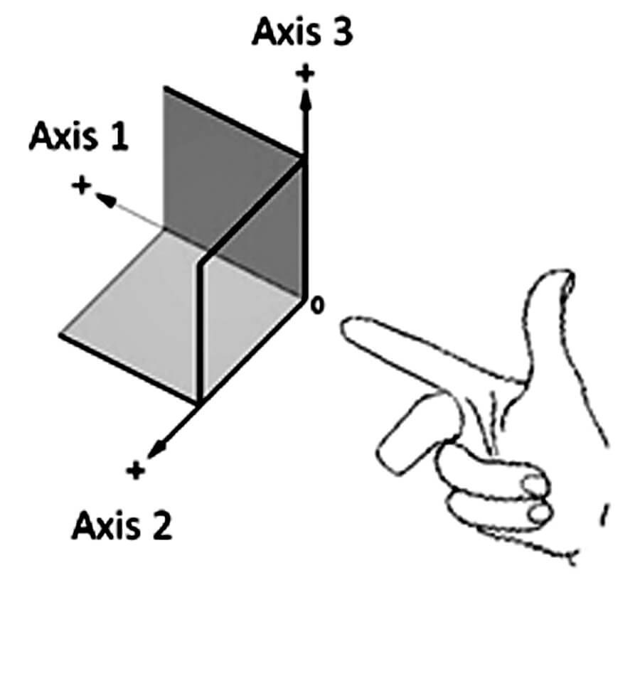
The orientation of the axes is defined by the right‐hand rule, where the first axis of the three points along the index finger, the second axis points along the middle finger and the third axis points along the thumb (Figure 3A).

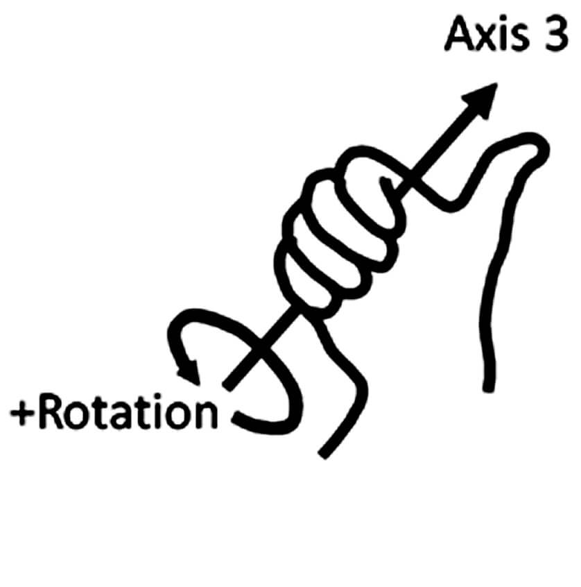
The rotation for this system occurs about Axis 3. The positive direction of rotation of the axis is also defined by the right hand rule where the thumb of the right hand points along the positive direction of Axis 3 and the curled fingers of the right hand indicate the positive angle of rotation (Figure 3B).

These relationships must be observed when defining the positive move directions for both the virtual and physical axes. The mapping from input to output axes starts with the virtual coordinate system and works back to the physical. At each step of the process the positive move directions of the mapped axes must be consistent with each other AND the right‐hand rule.

The orientation shown in Figure 4 is one of four that are possible. The other three are attained by rotating the x/y plane at intervals of 90 degrees around the z axis. The names of the axes in either system can be changed to meet application requirements. 

VERY IMPORTANT: The definition of positive motion of the axes is fixed based on the directions that the arrows are pointing in the illustration. Once the coordinate frames have been set‐up the positive move directions of the axes or part program must be changed to be consistent with the directions indicated by the coordinate frames.

Per the mapping we have defined in Figure 4, with no rotations active, motion in the +x direction would result in motion in the +X, motion in +y will result in +Y and +z will result in +Z.

Setting‐Up the TransformationConfigure() Function

A maximum of 32 matrix transformations can execute at the same time. In this case, the TransformationConfigure() function will configure the transformations and transform data from one three‐axis Cartesian system (InputAxes) into another three‐axis system (OutputAxes). Up to 512 matrices can exist simultaneously in each TransformationConfigure() function. This example will only require one TransformationConfigure() function to be configured for multiple matrices.

For the system shown in Figure 4, the first rotary axis is the B-axis and it rotates in the z/x plane about the y-axis of our input plane. Positive rotation motion will be counter‐clockwise per the right hand rule. The next rotary axis is the C-axis which rotates the x/y plane about the z-axis. Positive rotation motion will also be counter‐clockwise. The rotation matrices are specified as follows:

MatrixCreateRotateJ(B) – Creates a rotation matrix that rotates about the second input axis – y; the angle is determined by the rotary axis – B

MatrixCreateRotateK(C) – Creates a rotation matrix that rotates about the third input axis – z; the angle is determined by the rotary axis – C

So the TransformationConfigure() function for rotation matrices is shown below:

TransformationConfigure(0, [MatrixCreateRotateJ(B), MatrixCreateRotateK(C)], [x, y, z], [X, Y, Z])

[x, y, z] are the input axes, defined by the three virtual axes of the part positions. [X, Y, Z] are the output axes, defined by the three physical axes of the linear servo-system positions.

Setting‐Up Offsets

In most applications the center of rotation of the rotary axes are offset from each other. Additionally, the origin of the part coordinate system might not be located directly on the center of the axis of rotation as shown in Figure 5. The MatrixCreateTranslate() matrix is used to define the offsets between the axis of rotations and the part coordinate systems. The displacement command has offset values for all three axes. The offset is calculated based on the distance from the reference point to the rotation point. The sign of the displacement is based on the direction of movement from the reference point to the rotation point.

Using our example system, assume that the B and C axes of rotation intersect, the part origin is offset 15 mm above the tabletop of the C-axis and offset by 10 mm in the x direction, and the B-axis center of rotation is parallel to and in‐line with the y-axis and located 12 mm above the y-axis. Based on this configuration the offsets for the rotation commands would be as shown in Figure 5.

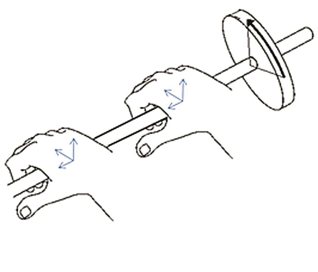
To calculate the offsets for the B-axis rotation about y-axis, the coordinate frame for the B-axis must be placed on its axis of rotation. The origin of this coordinate frame can be anywhere along the axis of rotation as the angular position along the B-axis does not change as a function of where the origin of rotation is located. For example, if a round pipe is rotated about its center, the angular position of any point on the pipe does not change based on the point along the pipe where the rotation is applied (Figure 6).

We can therefore place the origin of the point of rotation of the B-axis directly above the point of rotation of the C-axis which gives an offset of “0” in the x and y directions. The z offset is +12 as we move in the +z direction from the location of our starting point on the surface of the C-axis up to the B-axis of rotation. The offsets are placed in the order that the axes are defined in the MatrixCreateTranslate() matrix. The MatrixCreateTranslate() for the first rotation for B-axis:

MatrixCreateTranslate(0, 0, 12)

The offsets for the C-axis rotation are calculated in a similar fashion. From the illustration, the distance from the Part Origin to the center of rotation of the C-axis along the x-axis direction is +10. Along the z-axis direction the distance from the Part Origin to the center of rotation is -15. The Part Origin is in line with the y-axis so the offset in this direction is 0.

To set up the offset for the rotation for C-axis:

MatrixCreateTranslate(10, 0, -15)

After applying the offsets matrices to the same TransformationConfigure() function, the final TransformationConfigure() function is shown:

TransformationConfigure(0, [MatrixCreateRotateJ(B), MatrixCreateTranslate(0, 0, 12), MatrixCreateRotateK(C), MatrixCreateTranslate(10, 0, -15)], [x, y, z], [X, Y, Z])

Note that the MatrixCreateTranslate() matrices are placed in a specific order such that the offset is applied to its corresponding rotation matrix. In this example, MatrixCreateTranslate(0, 0, 12) is placed right after MatrixCreateRotateJ(B) because it is the offset calculated for the B-axis rotation.

After the transformation function is configured, the transformations are enabled/disabled with the following commands:

TransformationEnable()
TransformationDisable()

Issues with Constant Velocity/Surface Speed

When contouring is active in Automation1 with VelocityBlendingOn() function, the control will ramp‐up the vector velocity based on the task acceleration parameters until it reaches the programmed vector velocity given by the “F” code. This velocity will be maintained throughout the program until a condition that forces a deceleration is encountered. Maintaining constant velocity on the part has significant implications for the motion of the servo axes as they may be required to change speed or direction instantaneously.

The “standard” look‐ahead which monitors acceleration in an arc or detects a non‐tangent move between two program lines will not directly address this problem as the accelerations are produced indirectly by the Transformation function. There are two additional approaches that can be used to limit the acceleration of the physical axes.

The first method is to use a filter on the velocity command stream of the servo axes. The filter will have an effect similar to ramping, but it will also add a delay to the profile which will cause the path to deviate from the programmed path. The TrajectoryFIRFilter sets the length of an FIR (Finite Impulse Response) filter applied to the velocity command stream. Each “tap” in the filter equates to a 0.125 millisecond time interval. To add 50 milliseconds of filtering, the parameter would be set to 50/0.125 = 400.

The second method for reducing acceleration is to set the dependent axis acceleration limit. The B and C axes are considered dependent axes as their velocity command is derived from the virtual x/y/z axes. Short move-time for the x/y/z axes coupled with longer moves on the B/C axes can result in very high speed for the B/C axes. The SetupDependentCoordinatedAccelLimit() function can be used to limit the acceleration and resulting speed of the dependent axes.

Example Program

Following is a simple example that shows all of the commands in sequence and includes setup for acceleration limiting on the dependent axes.

program TransformationDisable(0) //Reset and disable the Transformation function Enable ([X, Y, Z, x, y, z, B, C]) Home ([X, Y, Z, x, y, z, B, C]) VelocityBlendingOn() //Enables velocity profiling mode SetupDependentCoordinatedRampRate(500) //Setup the coordinated accel and decel rate SetupDependentCoordinatedAccelLimit(4000) //Setup the acceleration limit on the dependent axes SetupTaskTimeUnits(TimeUnits.Seconds) //Set the feedrate to distance units per second F100 //Specify the feedrate of the dependent axes for coordinated motion G90 //Configure Absolute Positioning Target Mode /*Start configuring the Transformation Matrices [x, y, z] are the input axes; [X, Y, Z] are the output axes. MatrixCreateRotateJ rotates an angle about the second input axis – y; the angle is determined by the rotary axis – B MatrixCreateRotateK rotates an angle about the third input axis – z; the angle is determined by the rotary axis – C MatrixCreateTranslate defines the offsets values for the input axes */ TransformationConfigure(0, [MatrixCreateRotateJ(B), MatrixCreateTranslate(0, 0, 12), MatrixCreateRotateK(C), MatrixCreateTranslate(10, 0, -15)], [x, y, z], [X, Y, Z]) //Move physical X/Y/Z to the starting location G0 X5 Y60 Z23 //Move rotary axes to starting location G0 B0 C0 //Move virtual axes to starting location G0 x9 y0 AppDataCollectionSnapshot() //Start rotational transformation TransformationEnable(0) G1 x10 y2 z1 B3 C2 G1 x12 y3 z1.4 B3.7 C2.5 G1 x9 y2 z1.8 B3.8 C1.5 G1 x8 y2 z2.2 B0 C0 TransformationDisable(0) AppDataCollectionStop() VelocityBlendingOff() end

Reference Material

• Transformation Functions (aerotech.com)
• DefaultDependentCoordinatedAccelLimit Parameter (aerotech.com)
• TrajectoryFirFilter Parameter (aerotech.com)
• AxisType Parameter (aerotech.com)
• Lookahead Synchronization (aerotech.com)